Passive components
Table of contents
- Definition
- Components
- A generalization: impedance
- Even more general: two-port networks
- Size and scaling
Definition
Passive components are the fundamental building blocks of basic circuits. Their behavior is entirely described by simple, linear laws.
An active component, such as a transistor, has complex non-linear laws and can make a circuit’s behavior change radically over time.
In general, an electrical system can be charactized with 4 local quantities:
| Name | Symbol | SI units |
|---|---|---|
| Charge | $q$ | Coulomb (C) |
| Current | $i$ | Ampere (A) |
| Voltage | $V$ | Volt (V) |
| Magnetic flux | $\varphi$ | Weber (Wb) |
Here is a chart summarizing relationships between those 4 properties, and the 4 types of passive component that can act on them:

Components
Resistors

The most basic component by far. Its law simply expresses that passing current through it dissipates energy, in the form of heat:
\[V = Ri\]where $R$ is the resistance in Ohm (\Omega).
In resistive heaters, that heat is desirable (and 100% efficient!), but in any other application, it’s parasitic. The power consumption of a resistor is given by:
\[P = VI = \frac{V^2}{R} = Ri^2\]Two special cases of resistors are useful to keep as a mental model:
- $R \rightarrow \infty$: open circuit, any voltage can exists, but the current is always zero.
- $R \rightarrow 0$: ideal conductor, any current is allowed, but the voltage is always zero.
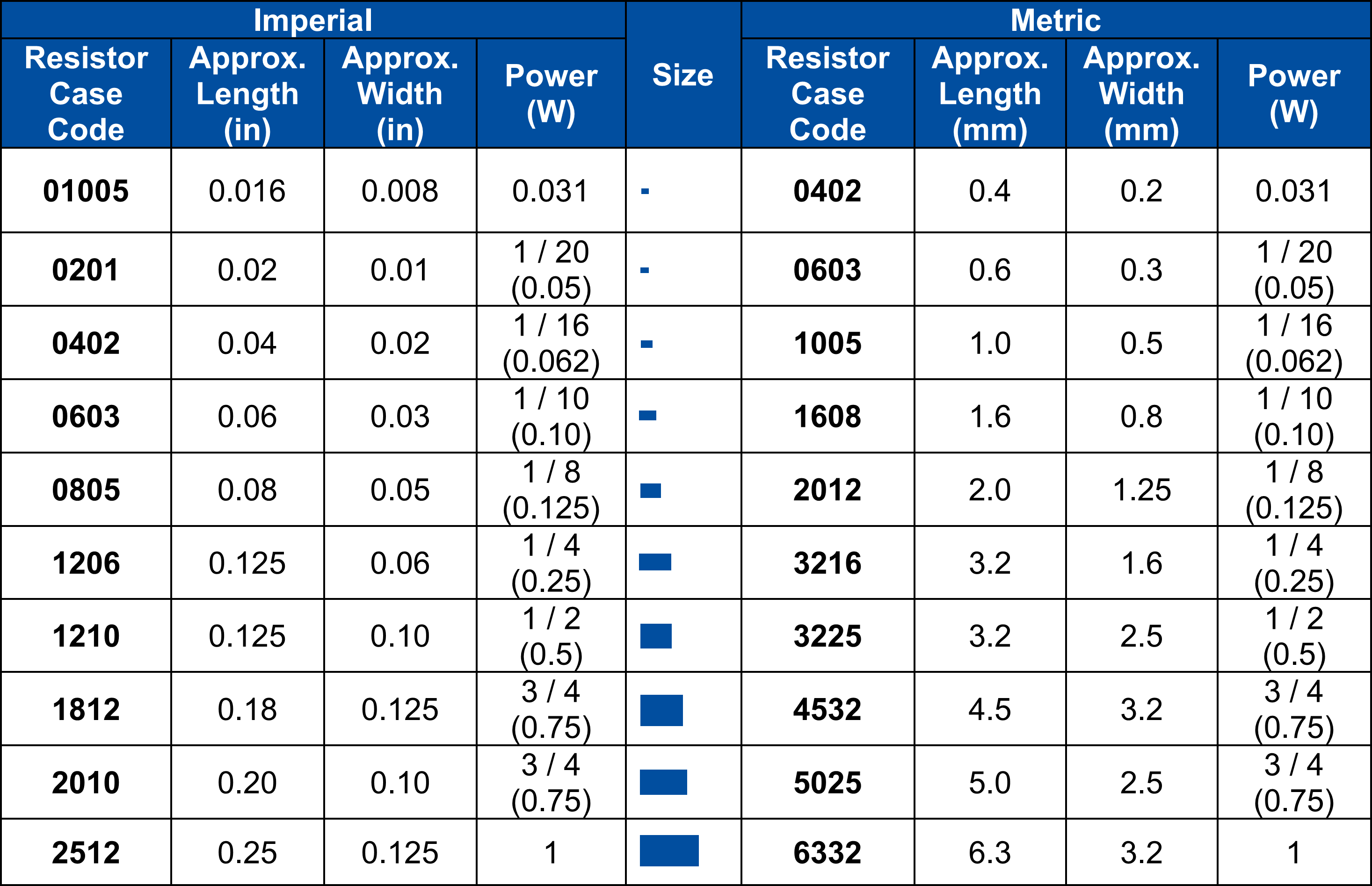
Resistors are the most common component in a circuit, and exist in many flavors:

The operation of a resistor is limited by the power it can handle. This power should be reduced if possible, but this is sometimes not an option. You can then move to bulkier resistor packages, capable of dissipating more heat. Here’s a handy chart:
Capacitors
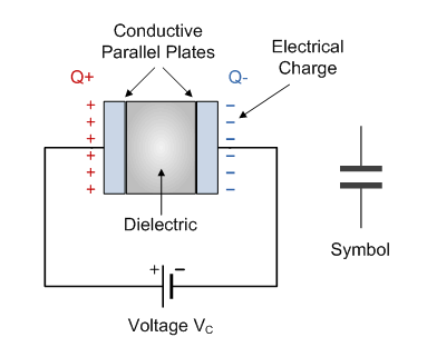
Capacitors are devices designed to store charge. The stored charge can be related to the voltage across its terminals by this simple law:
\[q = CV\]where $q$ is the charge, and $C$ the capacitance, expressed in Farad (F). Taking a time derivative gives a voltage/current law:
\[i = C \frac{\mathrm{d}V}{\rm dt}\]In the Fourier domain, this can be expressed as:
\[I(\omega) = j\omega C V(\omega)\]which reveals the (complex) impedance of a capacitor:
\[Z_c = \frac{1}{j\omega C}\]A capacitor behaves like a open circuit at frequency 0 (=DC), and a closed circuit at infinite frequencies. In other words, current is only allowed to exist in the presence of a transient in voltage. When the applied voltage stops changing, the capacitor will eventually charge to perfectly compensate it, stopping the passage of current.
In practice, capacitors can serve one of several roles in a circuit. Common ones are:
- Decoupling: serve as a local power source to dampen current consumption spikes from devices. It’s common to place decoupling capacitors next to every IC in a circuit (~1uF), and to have larger capacitors for decoupling the entire board from the power supply.
- Filtering: combined with a resistor, a low-pass (or high-pass) filter can be built, with use in signal processing or power management (see rectifiers).

source: https://eeeproject.com/types-of-capacitors/
There are various types of capacitor to pick from. Main types are:
- Non-polarized:
- ceramic: most common, uses ceramic as the dielectric. Can tolerate high voltages, but capacitance doesn’t go much higher than 100uF.
- film: uses a plastic film as the dielectric. Advantages include high precision and stability.
- Polarized:
- Electrolytic: medium-high values. The dielectric used is the thing oxide layer forming on the metal anode (e.g. aluminum, tantalum). Disadvantages include poor value tolerance and leakage current. as the dielectric
- Super capacitor: highest values, but only usable at low voltage.
They also show up spontaneously in circuits, and need to be modeled accordingly. Any conductor pair acts as a capacitor, even the cable coming from your power supply, or differential data pairs. Parasitic capacitance, combined with parasitic resistance, is what limits (very) high frequency operation of most circuits.
When picking a capacitor, the one most important metric is the voltage rating (or breakdown voltage). Beyond that, sparks begin to form between the electrodes, turning the capacitor into a short circuit.
Temperature also comes into play, as it can change the dielectric constant of the insulator. Here is a good reference about capacitor rating codes: https://www.allaboutcircuits.com/technical-articles/x7r-x5r-c0g…-a-concise-guide-to-ceramic-capacitor-types/
Inductors
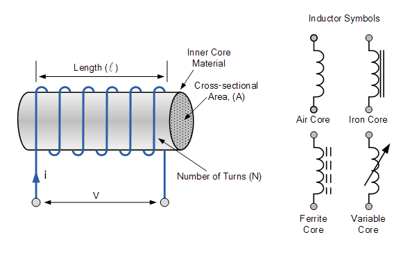
Inductors relate magnetic flux and current. Any passage of current through a conductor generates a magnetic field around it; inductors are simply designed to maximize this magnetic field. Their fundamental law is:
\[\varphi = L i\]where $\varphi$ is the magnetic flux passing through the inductor, and $L$ is the inductance, expressed in Henry (H). Taking a time derivative gives a direct relationship between the current and the voltage across it (equal and opposite to the induced electromotive force):
\[V = L \frac{\mathrm{d}i}{\rm dt}\]or in the Fourier domain:
\[V(\omega) = j\omega L I(\omega)\]showing that the impedance of an inductor is given by:
\[Z_L = j\omega L\]At a zero frequency, an inductor is equivalent to an ideal conductor, while at infinite frequencies, it behaves like an open circuit. In other words, rapid changes of current are not allowed due to the inertia of the magnetic flux.
There are many types and sizes of inductors, depending on the application:

Types of inductor include:
- Air core: just a coil, can only provide small inductance values.
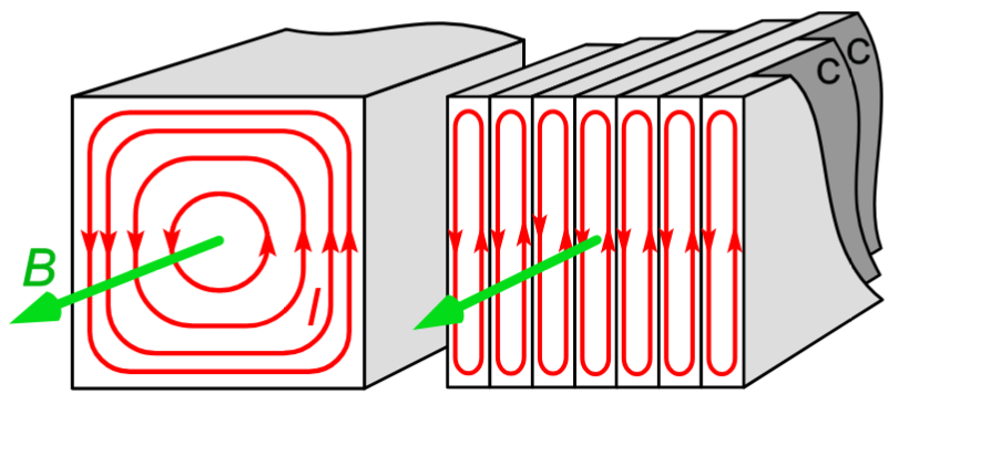
- Iron/ferrite core: higher inductance values, used for high performance inductors and transformers. Eddy currents (i.e. heat losses in the core) can be reduced by using a laminated (layered) core.
- Toroidal: the core is donut-shaped, forming a closed loop that fully contains the magnetic fields. Higher inductance values are possible, but they are harder to fabricate.
- PCB coil: a simple spiral on a PCB. Only low inductance can be achieved, but this manufacturing method is as cheap as it gets.
Recently, 3D printed inductors have shown to be viable: https://news.mit.edu/2024/mit-engineers-3d-print-electromagnets-solenoids-0223
The operation of an inductor is limited by their maximal current and voltage. When the voltage gets too high, the insulator in the windings can no longer prevents sparks from forming, causing short circuits and damage. When the current is too high, the parasitic resistance of the coil starts to show, and temperature builds up.
Heat losses in the core are caused by Eddy currents: the induced current in the core is subject to resistive heat losses. This can be mitigated by using a laminated core:
Memristors
The elusive memristor was first proposed by prof. Chua in 1971, as being the missing 4th type of passive component. Its law would relate electric charges and magnetic flux:
\[\varphi = M q\]Memristors are still actively being researched, Hewlett Packard claiming to have developed the first one in 2008. They might do a comeback soon, due to rumored applications in AI chips.
A generalization: impedance
Any series/shunt combination of passive components can be summarized by a generalized law in the Fourier domain:
\[V(\omega) = Z I(\omega)\]where $Z$ is the (complex) impedance, and can be expressed as:
\[Z = R + j X\]with $R$ being the resistance, and $X$ the reactance, caused by capacitors and/or inductors present in the mix. While $Z$ is overall expressed in Ohms, only its real part causes dissipative losses. The reactance has a net power of zero, as its isolated contribution is a +/-90° phase offset between the voltage and current, causing an average power of zero over time.
The inverse of an impedance is called admittance, and can be summarized as:
\[Y = G + j B\]where $G$ is the conductance, and $B$ the susceptance, expressed in Siemens (1S=1/Ohm).
Even more general: two-port networks
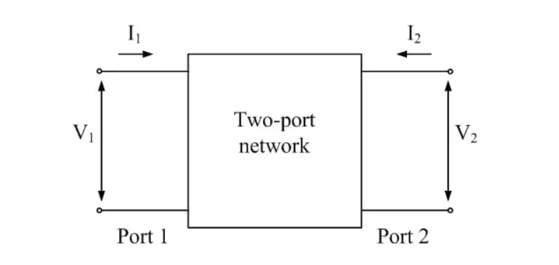
The two-port network is a model that can prove very useful when trying to isolate and fully describe a part of a circuit, that has identifiable input and output terminals. In the two-port representation, the input voltage/current pair is related to the output voltage/current pair by the following law:
\[\begin{bmatrix}V_1 \\ V_2\end{bmatrix} = \begin{bmatrix}z_{11} & z_{12} \\ z_{21} & z_{22}\end{bmatrix} \begin{bmatrix}I_1 \\ I_2\end{bmatrix} := [z] \begin{bmatrix}I_1 \\ I_2\end{bmatrix}\]The impedance matrix can be found by setting $I_1=0$ or $I_2=0$ and analyzing $V_1$ and $V_2$:
\[z_{11} := \left.\frac{V_1}{I_1}\right|_{I_2=0} \qquad z_{12} := \left.\frac{V_1}{I_2}\right|_{I_1=0}\] \[z_{21} := \left.\frac{V_1}{I_1}\right|_{I_2=0} \qquad z_{22} := \left.\frac{V_1}{I_2}\right|_{I_1=0}\]Alternatively, the currents can be described as a function of the voltages using the admittance matrix:
\[\begin{bmatrix}I_1 \\ I_2\end{bmatrix} = \begin{bmatrix}g_{11} & g_{12} \\ g_{21} & g_{22}\end{bmatrix} \begin{bmatrix}V_1 \\ V_2\end{bmatrix} := [g] \begin{bmatrix}V_1 \\ V_2\end{bmatrix} = [z]^{-1} \begin{bmatrix}V_1 \\ V_2\end{bmatrix}\]The ABCD representation mixes current and voltages and is handy when cascading systems:
\[\begin{bmatrix}V_1 \\ I_1\end{bmatrix} = \begin{bmatrix}A & B \\ C & D\end{bmatrix} \begin{bmatrix}V_2 \\ -I_2\end{bmatrix} := [a] \begin{bmatrix}V_2 \\ -I_2\end{bmatrix}\]Two-port models can be elegantly combined:
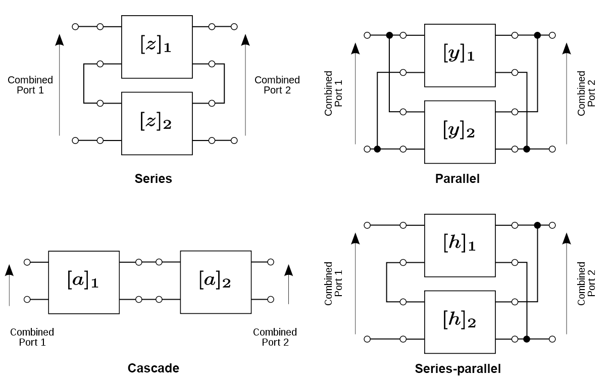
For example, in the series configuration, the combined impedance matrix is given by:
\[[z]_{\rm series} = [z]_1 + [z]_2\]In the parallel configuration, the combined admittance matrix is:
\[[g]_{\rm admittance} = [g]_1 + [g]_2\]In the cascade configuration, the ABCD matrices can be combined through matrix multiplication:
\[[a]_{\rm admittance} = [a]_1 [a]_2\]Size and scaling
Inductors and capacitors are the critical energy storage elements needed for power conversion. Miniaturization has driven these passive components to become smaller and smaller. Capacitors are relatively easy to miniaturize. Building a capacitor using traces on a PCB is a good trick. Inductors on the other hand are difficult to miniaturize. The following analysis is for passives, but apply also to actuators (consider the co-energy)!
Magnetics scale poorly with decreasing size
The scaling of magnetics was first published by Sullivan et al. The analysis presented here is taken from 6.332 course notes by Prof. Dave Perreault.
Magnetics are often the largest and most lossy components of a power converter (often responsible for half the loss and take up half the volume). Fundamental physics make the miniaturization of magnetics a challenge.

The power handling or “volt-ampere” of an inductor driven at a sinusoidal frequency $f$ is
\[\textrm{Power Handling} = V\cdot I = (2\pi f \underbrace{N B_0 A_C}_{\lambda}) \left(\frac{J_0 W_A}{N}\right)\] \[\textrm{Power Handling} = 2\pi f B_0 J_0 (A_C W_A)\]With all else equal, consider scaling the length by a factor $s$. The power handling then scales as
\[\textrm{Power Handling} \propto (A_C W_A) \propto s^4\]whereas the volume scales with $s^3$. Therefore the power handling per volume scales as
\[\frac{\textrm{Power Handling}}{\textrm{volume}} \propto s\]which reduces at small scales! This is why shrinking magnetics is hard. The power handling ability of your magnetics shrinks faster than the volume!
Notice that power handling scales proportionally with frequency. This is why in the race to bottom, designs are pushing to ever higher and higher frequencies. In real systems, at large scales the performance tends to be limited by $B_0$ or the saturation of the iron and at small scales the limitation is in $J_0$ due to heat.
Electrostatics scale nicely with decreasing size
In contrast, if we consider power handling of a capacitor
\[\textrm{Power Handling} = V\cdot I = (V)(2\pi f C V)\] \[\textrm{Power Handling} = 2\pi f C V^2 = 2\pi f \epsilon V^2 \left(\frac{A}{d}\right) \propto s\]We find the capacitance $C=\epsilon \frac{A}{d}$ scales with $s$ and therefore
\[\frac{\textrm{Power Handling}}{\textrm{volume}} \propto s^{-2}\]This is why capacitors and electric field systems are so ubiquituous on silicon and MEMS!